


A cluster won’t be fully utilized until you set enough parallelism for every operation. All of this ties back one way or another to the number of partitions.
The usual Spark advice is to keep about four times as many partitions as there are cores in the cluster. There’s also an upper bound on that number, set by task runtime — each task should run for at least 100ms. If tasks finish faster than that, your partitions are probably too small, and Spark will spend more time handing out tasks than doing the actual work.
Too few partitions and too many are both bad, each in their own way:
Too few partitions and you’re not using all the available cores in the cluster.
Too many partitions and extra overhead managing a pile of tiny tasks and moving data around.
If you’re still unsure, it’s safer to have more tasks (and partitions) than fewer.
These recommendations are useful, but you’ll still have to tune Spark’s settings for your specific scenario to make the application as optimal as possible.
So what actually affects partitioning?
Once you get into the details of working with Spark, it’s important to understand these parts of your pipeline, because they affect how you’ll partition your data:
Business logic
Data
Environment
Let’s walk through each area and see how it relates to partitioning.
Business logic
Let’s start with business logic. It varies enormously, so specific advice is hard here: every pipeline is different, and I haven’t seen yours (which is probably for the best).
Reduce the size of the working dataset
The most effective advice is usually the dumbest — to speed up the application, reduce the amount of data the Spark cluster has to process. There are several ways to do that, and of course it all depends on what actually needs doing with the data.
First rule of data engineering: the fastest data is the data you didn’t read. Filter as early as you can, and correct partitioning will let Spark honestly ignore almost everything sitting on disk.
You can filter the source data by skipping partitions that don’t match your predicate — the right filter can speed up reading and fetching data a lot. Sometimes, as with S3, you can avoid unnecessary partition discovery, and partition pruning skips whole directories the predicate can’t match. Both assume somebody partitioned the data sensibly. (Strong assumption, I know).
Repartition before multiple joins
join is one of the most expensive and most common operations in Spark, primarily because of the shuffle it triggers. Shuffle is a big topic, but here I’ll focus on how it relates to partitions.

To join data, Spark needs rows with the same join key to sit in the same partition. The default join implementation in Spark since version 2.3 is sort-merge join.
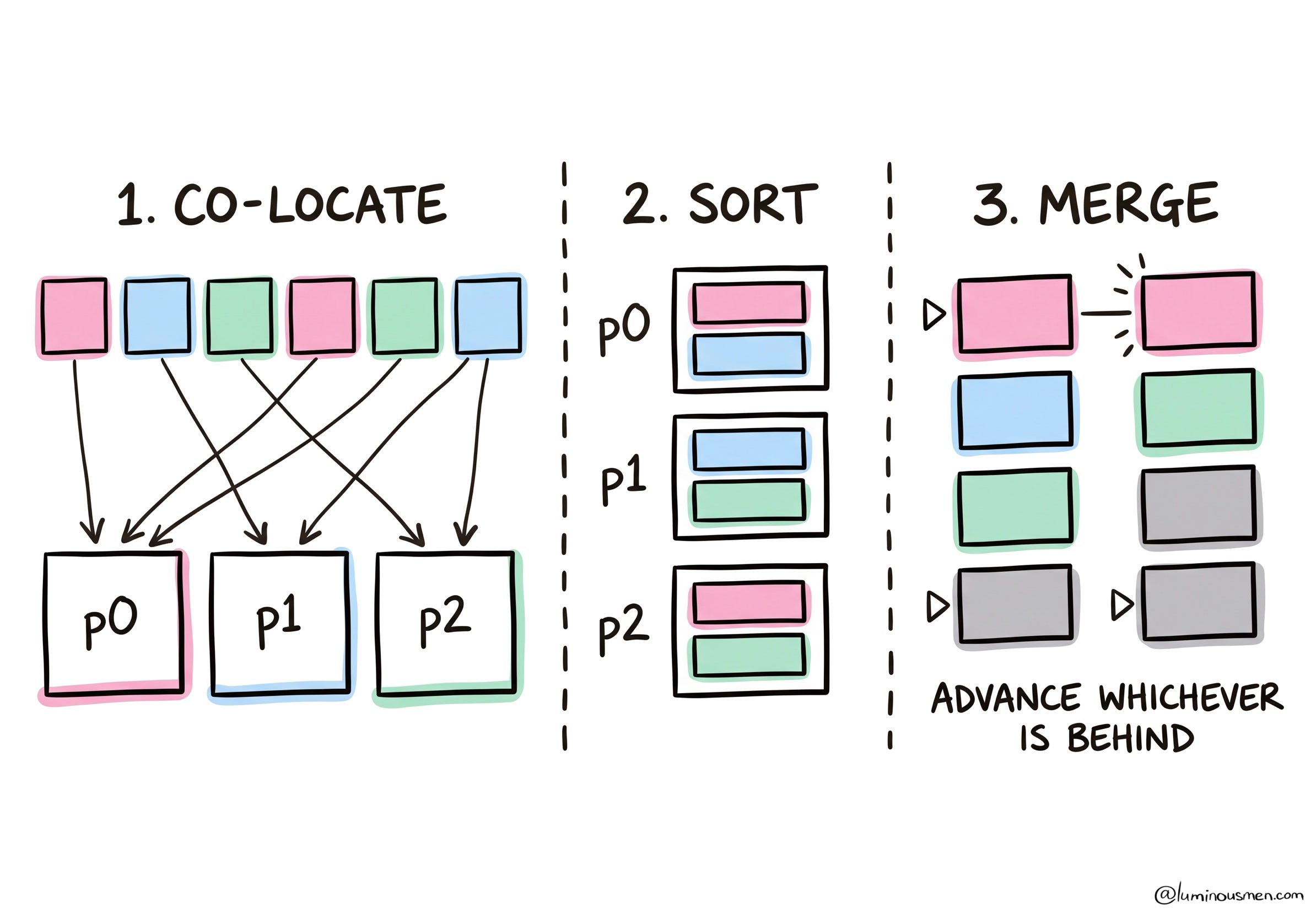
Sort-merge join runs in three basic steps:
Bring the data together. Rows with the same key have to end up in the same partition, and that’s a shuffle.
Sort the data inside each partition, in parallel.
Merge them. Both sides are sorted by now, so Spark reads them side by side, advancing whichever side is behind and gluing rows together when the keys match. That’s what step 2 was for.
Shuffle in step 1 is expensive, and you don’t always need it. You can technically skip it when:
Both sides are already partitioned the same way on the join key — because you repartitioned them yourself, or because the tables are bucketed.
One side is small enough to fit in memory, in which case Spark will take a broadcast hash join instead.
As an example, if you know a dataframe will need to be joined several times, you can avoid the extra shuffling by repartitioning it yourself. Just don’t forget to cache the dataframe after.
users = spark.read.load('/path/to/users')
users = users.repartition('userId').cache()
joined1 = users.join(addresses, 'userId')
joined1.show() # 1st shuffle for repartition
joined2 = users.join(salary, 'userId')
joined2.show() # skips shuffle for users since it's already been repartitioned
Repartition after flatMap
After a flatMap you usually end up with more rows: unlike map, which returns exactly one output row per input row, flatMap returns a collection per input row, and Spark flattens those collections into the output rows. One input row easily becomes ten, or a thousand. And flatMap is a narrow transformation: there’s no shuffle, partition boundaries don’t move, and number of partitions don’t change. Spark can’t rebalance anything up front either — it doesn’t know how many rows your function will return until it runs it.
The result is that the same 200 partitions now carry way more data: each partition’s memory gets overloaded, disk spills start, and so does garbage collection pauses. Better to repartition the output of flatMap, scaled to how much the data grew.
Get rid of disk spills
From the Tuning Spark docs:
Sometimes, you will get an
OutOfMemoryError, not because your RDDs don’t fit in memory, but because the working set of one of your tasks, such as one of the reduce tasks ingroupByKey, was too large. Spark’s shuffle operations (sortByKey,groupByKey,reduceByKey, join, etc) build a hash table within each task to perform the grouping, which can often be large ...
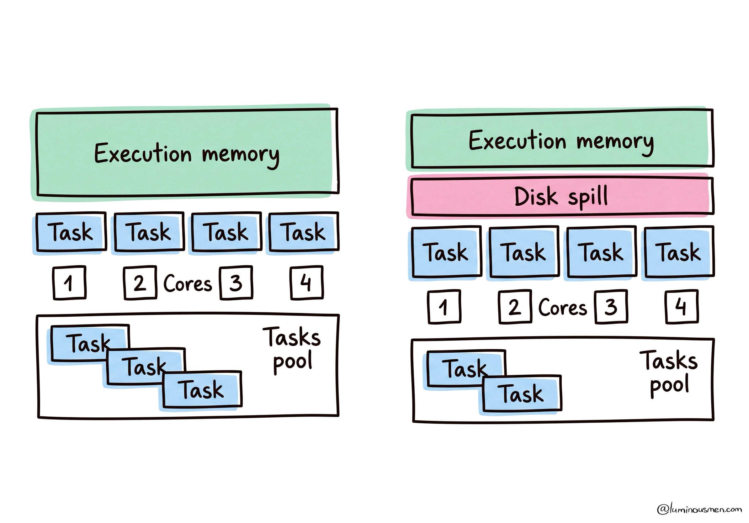
If spark.shuffle.spill is on (and it is by default), Spark uses ExternalAppendOnlyMap during shuffles to store intermediate data. When there isn’t enough memory, this structure spills data to disk, which adds pressure on executor memory and leads to extra disk I/O and more frequent garbage collection.
PySpark makes it even worse. Python workers live outside the JVM heap and take their memory from spark.executor.memoryOverhead, which defaults to 10% or 384MB. So the JVM spills while Python just grows, until YARN or Kubernetes kills the container and you find nothing useful in the logs.
To check whether a disk spill happened, you can search the logs for entries like this:
INFO ExternalSorter: Task 1 force spilling in-memory map to disk it will release 232.1 MB memoryThere are a few ways to fix this:
Reduce the volume of data: select only the columns you need, for example, or move filtering ahead of the wide transformations.
Raise the level of parallelism so each task’s input is smaller. Or manually
repartition()before the stage.Increase the shuffle buffer by raising executor memory (
spark.executor.memory). Look at how Spark splits the heap between execution and storage.If you have the memory, you can increase
spark.shuffle.file.bufferso the buffers overflow less often on the shuffle write — that reduces the number of disk I/Os.
You can find more configuration optimization options with this tool.
Data
When you work with data, understanding your data is the baseline. If you try to tune a Spark application without knowing your own data, you’ll most likely end up with bad performance and wasted resources.
Data skew
Ideally, when Spark does a join, the join keys should be spread evenly across partitions. But real data is usually faaaar from ideal: some keys have a handful of records, others have tens of millions.
This isn’t just a Spark disease. Skew breaks any distributed system — Flink, a sharded database, good old MapReduce. The moment work is split by key, uneven keys turn into uneven load, which turns into one node doing all the work while the rest just wait.
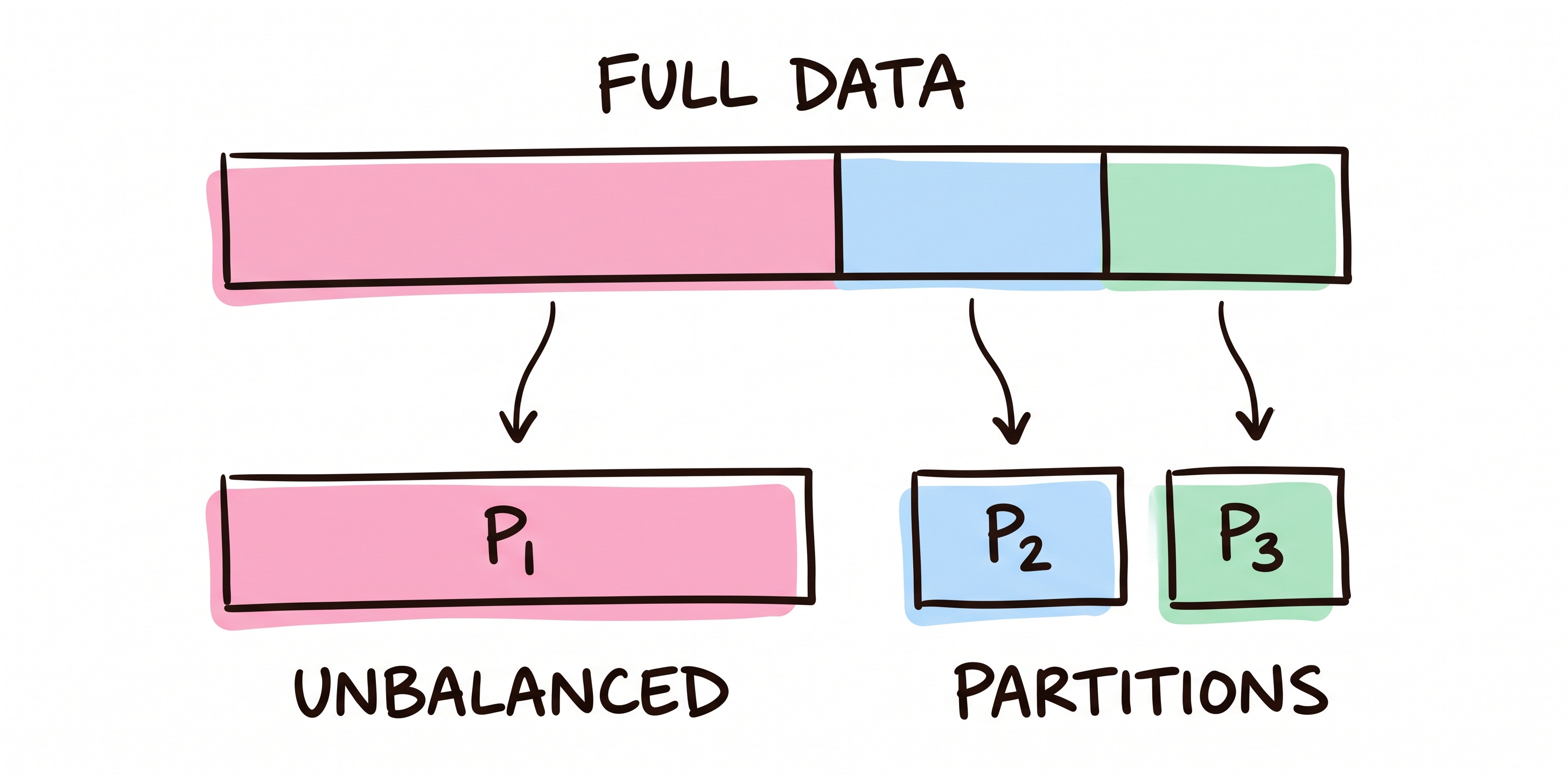
It shows up everywhere there’s grouping by key: in joins, in groupBy, in the file layout on disk. You partitioned by country, and the USA partition weighs as much as all the others combined. One partition like that sets the runtime of the whole stage, because a stage isn’t done until its slowest task is. You’re paying for the whole cluster and one core is working.
Let’s look at some code, for example:
import pandas as pd
import numpy as np
from pyspark.sql import functions as F

# set smaller number of partitions so they can fit the screen
spark.conf.set('spark.sql.shuffle.partitions', 8)
# disable broadcast join to see the shuffle
spark.conf.set("spark.sql.autoBroadcastJoinThreshold", -1)
length = 100
names = np.random.choice(['Bob', 'James', 'Marek', 'Johannes', None], length)
amounts = np.random.randint(0, 1000000, length)

# generate skewed data
country = np.random.choice(
	['United Kingdom', 'Poland', 'USA', 'Germany', 'Russia'],
	length,
	p = [0.05, 0.05, 0.8, 0.05, 0.05]
)
data = pd.DataFrame({'name': names, 'amount': amounts, 'country': country})
transactions = spark.createDataFrame(data).repartition('country')
countries = spark.createDataFrame(pd.DataFrame({
	'id': [11, 12, 13, 14, 15],
	'country': ['United Kingdom', 'Poland', 'USA', 'Germany', 'Russia']
}))
df = transactions.join(countries, 'country')

# check the partitions data
print(df.rdd.glom().map(len).collect())
One partition out of eight took 82 rows out of 100, and four are completely empty — that smells like skew.
💡 In a real pipeline glom() won’t help — the dataset won’t fit in the driver. You have to look at the Spark UI, Stages tab: for every stage there’s a distribution of task times by quantile. If the max is several times the median, that’s skew. The same symptom from the other side: 199 tasks out of 200 went green a while ago and the stage is still hanging on one.
What to do about it, in increasing order of effort:
Redistribute the data onto more evenly distributed keys, or just increase the partition count
Broadcast the smaller dataframe, if that’s possible
Use an extra random key to spread the data better (salting)
Differential replication
Iterative broadcast join
Now let’s go through each one in more detail.
Repartitioning
The most obvious fix is to redistribute the data with an explicit repartition. It helps when the problem is the partitioning, not the data: there are too few partitions, or the partitioning key was chosen poorly, while the keys themselves are distributed more or less evenly.
But it won’t save you from a hot key. Every row with country = 'USA' will go to one partition no matter how many partitions there are — that needs the tools below. Aside of that, repartition is always a shuffle, so you don’t drop it in blindly, “just in case”.
Broadcast the smaller dataframe
The shuffle is also what produces the skew: every row with the hot key ends up in the same partition.
Broadcast join removes the shuffle, and the skew with it. If one of the tables is small, Spark collects it on the driver and sends a copy to every executor. From there each executor joins its slice of the big table against its local copy of the small one — nothing travels over the network, there’s no shuffle at all.
df = transactions.join(F.broadcast(countries), 'country')
F.broadcast() is a hint, not a command: Spark ignores it when the join type can’t be broadcast. But it does override spark.sql.autoBroadcastJoinThreshold — the hinted side gets broadcast whatever its size. Spark can also pick broadcast on its own, if the statistics tell it the table is under that threshold (10MB by default). The problem is that it often doesn’t have the statistics — for example, when one side of the join is the result of previous transformations.
Salting
The problem with skew is that Spark is too obedient: you told it to join by country, so it joins by country, and every transaction from the USA goes to one partition. One key, one partition, nothing to argue about.
So we need to change that step a little to spread the data out — we add a random number to the key, the salt, and USA becomes USA@0, USA@1, … USA@9. To Spark those are ten different keys, it honestly spreads them across ten partitions, and it never suspects it’s been tricked.
The small side of the join has to be replicated across every possible salt value as well. Otherwise the row USA@7 won’t find a match — the lookup table just has USA.
SALT_FACTOR = 10

# every lookup row is replicated across all salt values
salted_countries = countries.withColumn(
    'salt',
    F.explode(F.array([F.lit(i) for i in range(SALT_FACTOR)])))

# every transaction gets a random salt. cast('int'), not round:
# round would give SALT_FACTOR + 1 buckets, and the last one would have no match
salted_transactions = transactions.withColumn(
    'salt', (F.rand() * SALT_FACTOR).cast('int'))

df = (salted_transactions
      .join(salted_countries, ['country', 'salt'])
      .drop('salt'))

# check the partitions data
print(df.rdd.glom().map(len).collect())
The result is a noticeably smoother distribution across partitions: instead of one overloaded task, ten normal ones are working.
Differential replication
Salting works, but it’s a bit dumb: you set 10, and the whole lookup table inflates tenfold. The USA key, the one this is all about, got replicated ten times. The Poland key with its three rows — also ten times. We cured the skew by making everyone equally miserable.
Fair, I guess? Treat the patient, not the whole clinic. Differential replication does that: first we work out which key is actually the fat one, and replicate only that one heavily. Everyone else gets the minimum, just enough that their rows still find a match. Hot keys get their own policy, everyone else gets theirs.
replication_high = 7
high = F.broadcast(
	spark.range(replication_high)
		.withColumnRenamed('id', 'replica_id')
)
replication_low = 2
low = F.broadcast(
	spark.range(replication_low)
		.withColumnRenamed('id', 'replica_id')
)

# determine which keys are highly over-represented, broadcast them
skewed_keys = F.broadcast(
    transactions.freqItems(['country'], 0.6)
        .select(F.explode('country_freqItems').alias('country_freqItems'))
)

# replicate uniform data, one copy of each row per bucket
countries_skewed_keys = (
    countries
        .join(
            skewed_keys,
            countries.country == skewed_keys.country_freqItems,
            how='inner')
        .crossJoin(high)
        .withColumn('composite_key', F.concat('country', F.lit('@'), 'replica_id'))
)
countries_rest = (
    countries
        .join(
            skewed_keys,
            countries.country == skewed_keys.country_freqItems,
            how='leftanti')
        .crossJoin(low)
        .withColumn('composite_key', F.concat('country', F.lit('@'), 'replica_id'))
        .withColumn('country_freqItems', F.lit(None))
)

# this is now the entire uniform dataset replicated differently
countries_replicated = countries_skewed_keys.union(countries_rest)
transactions_tagged = (
    transactions
        .join(
            skewed_keys,
            transactions.country == skewed_keys.country_freqItems,
            how='left')
        .withColumn('replica_id',
            F.when(
                F.isnull(F.col('country_freqItems')),
                (F.rand() * replication_low).cast('int'))
            .otherwise((F.rand() * replication_high).cast('int')))
        .withColumn('composite_key', F.concat('country', F.lit('@'), 'replica_id'))
)

# now we can join on the composite key
df = transactions_tagged.join(countries_replicated, 'composite_key')

print(df.rdd.glom().map(len).collect())
Frequent keys get replicated frequently, and the rest get whatever’s left.You’ll pay for it in complexity. This is no longer “add a column with rand() and live in peace”, it’s two joins, a crossJoin, freqItems, and a composite key that then drags through the whole pipeline and surfaces at the worst possible moment.
Iterative broadcast join
The last resort, when the lookup table is too big to broadcast but you don’t want to shuffle it either. The idea here is to cut the smaller side into N chunks, broadcast each chunk separately and join it against the big table, then stack the results with union.
There’s no shuffle on any pass, which means no skewed partitions either. What you pay is N passes over the big table instead of one — which is why the technique only makes sense when N is small and the shuffle really is expensive.
Coalesce after filtering
As mentioned already, good filtering really does boost performance. But even if you squeeze 2 billion rows (2TB) across 15,000 partitions down to 2 million rows, the partition count stays the same. Most of those partitions will be empty and will still eat resources.
That’s where the coalesce operation comes in — it lets you reduce the number of partitions, and now is the perfect moment to use it.
df = huge_data.sample(withReplacement = False, fraction = 0.001)
df = df.coalesce(4)
This applies not only to filtering but to aggregation as well.
Environment
So far we’ve been looking inside the application — at the data and at what the code does with it. But the application doesn’t run in a vacuum. It runs on a specific cluster with a specific number of cores, it writes to specific storage that somebody else will later read from, and it pulls data out of systems that know nothing about Spark (and probably don’t want to).
All of that affects partitioning just as much as the data does.
Size your output files for the reader
Spark’s DataFrameWriter has a partitionBy method that splits the output across directories as it writes:
df.write.partitionBy('key').json('/path/to/foo.json')On disk you get directories like key=bar/ and key=baz/ instead of a single flat directory of files. The column value lives in the directory name now, not inside the files. The point here is that downstream jobs can avoid reading what they don’t need — when a query has a filter on that column, Spark simply won’t walk into the unneeded directories:
df = spark.read.schema(schema).json('/path/to/foo.json')
df.where(df.key == 'bar')
The reader matters more than the writer here. On write Spark creates one file per task, and on read it takes at least one file per task — and the size of those files is effectively something you impose on everyone who will read your data later. If a fat cluster with a lot of memory per executor did the writing, the partitions could have come out large; a smaller cluster that comes for this data tomorrow inherits those sizes, and with less memory per executor it spills them to disk or dies in OOM pain.
So write for the smallest cluster that will read this, not the one that wrote it. The reading side packs spark.sql.files.maxPartitionBytes (128MB by default) into each partition, so aim your file sizes at that — and when repartition isn’t a precise enough lever, spark.sql.files.maxRecordsPerFile caps it directly.
Repartition before writing to storage
Unlike repartition, partitionBy triggers no shuffle — it only decides which directory each row ends up in.
No shuffle — sounds great, right?
Great, until you look at the file count. Since there’s no shuffle, every task writes on its own and knows nothing about the others. Say we have 10 partitions and we’re splitting the output by day across a year: every task creates its own 365 files, for a total of 365×10=3650 per job. And if there are 200 partitions, as there are after a normal shuffle stage, that’s already 365×200=73 thousand. Hello, small files problem.
So the advice here is: before writing, repartition by the same columns you’re about to partition by.
(df.repartition('key')
   .write
   .partitionBy('key')
   .json('/path/to/foo.json'))
Now all the rows for one key sit in one partition, which means one task writes them, which means you get exactly one file per key. You’ll pay a shuffle for it — but one shuffle on write is cheaper than 73 thousand files that every subsequent job will be digging through until the end of time.
Use all the available cluster cores
The total core count is the absolute ceiling for available parallelism. If you have 200 cores and 10 partitions on read, 10 cores will be working but you’re paying for the other 190 without using them.
They also sit idle in a far less obvious case: tasks come in waves, so 3 partitions of a minute each on 2 cores will take not a minute and a half but two — the second wave is carried by one core while the other one stands still.
Hence the practical advice: keep the partition count a multiple of the core count, and preferably with headroom — those same 2–4 partitions per core from the start of the article. The multiple removes the under-loaded final wave, and the headroom gives the scheduler room to maneuver: if one task turns out heavier than its neighbors, the other cores will get through the queue while it finishes.
And bear in mind that on read you don’t set the partition count. It comes from the file layout and spark.sql.files.maxPartitionBytes (128MB by default), so ten large files will give you exactly ten partitions — and repartition() here will cost you a full shuffle.
Put a stage barrier between the shuffle stage and the write
There’s a non-obvious thing here: coalesce doesn’t shuffle, it just merges neighbouring partitions. No shuffle means no stage boundary, so the reduced count applies to the whole stage and not only to the write. Put coalesce(10) before the write and you wanted ten files but got ten tasks for all the processing.
The solution here is to create a stage barrier. The simplest option is to write the dataframe to temporary storage and read it back, but localCheckpoint is cheaper:
(df.localCheckpoint()
   .repartition(n)
   .write.parquet('/path/to/output'))
The barrier cuts repartition off from everything that came before it: the partition count won’t travel any further up, and a parallel workflow using the same dataframe won’t have to recompute it from scratch. Just bear in mind that Spark is lazy, and localCheckpoint() triggers execution right at that point in order to materialize the dataframe.
Partitioning with JDBC sources
Traditional SQL databases can’t spread processing across nodes the way Spark does. By default Spark reads a table into a single partition: one connection, one task, one executor working, the rest of the cluster watching.
With files Spark splits the work itself, because it can see the byte ranges. A table gives it nothing to split on, so the only way to read one in parallel is to send several queries with different WHERE ranges and let the database answer them side by side. Spark will write those queries for you, but it can’t guess the column to slice on or the range that column covers, so you have to hand it all four options at once:
df = (spark.read.format('jdbc')
      .option('url', url)
      .option('dbtable', 'transactions')
      .option('partitionColumn', 'id')
      .option('lowerBound', 0)
      .option('upperBound', 1000000)
      .option('numPartitions', 10)
      .load())
Spark will split the range lowerBound..upperBound into numPartitions chunks and send a query for each. Two consequences follow. First: the column has to be evenly distributed, otherwise you get the same skew, except now its cause is your own WHERE id BETWEEN. Second: numPartitions is the number of simultaneous connections to a production database. Two hundred parallel tasks against an OLTP database take down more than your job.
Why AQE doesn’t save you
Why bother doing everything by hand when we now have AQE?