If you've spent any time wrangling data at scale, you've probably heard of Apache Spark. Maybe you've even cursed at it once or twice — don't worry, you're in good company.
Spark has become the go-to framework for big data processing, and for good reason: it's fast, versatile, and (once you get the hang of it) surprisingly elegant. But mastering it? That's a whole other story. Spark is packed with features and an architecture that feel simple on the surface but quickly grow complex. If you've ever struggled with long shuffles, weird partitioning issues, or mysterious memory errors, you know exactly what I mean.
This article is the second in a series on Apache Spark, created to help you get past the basics and into the real nuts and bolts of how it works — and how to make it work for you.
Apache Spark Key Abstractions
At its core, Spark is built on two fundamental abstractions:
Resilient Distributed Dataset (RDD)
Directed Acyclic Graph (DAG)
These are the gears under the hood of everything Spark does. Let's unpack each one.
RDD — The Core of Spark
The beating heart of Apache Spark is the Resilient Distributed Dataset (RDD) — a collection of objects spread across cluster nodes for parallel processing. RDDs were Spark's original abstraction and still remain central to its design, even as DataFrames and Datasets have taken center stage.
💡 While RDDs are still there under the hood — especially when it comes to low-level fault-tolerant mechanics — you shouldn't write modern Spark code directly with RDDs. Unless you're doing something super low-level (like custom serialization or working with graphs), stick with DataFrames or Datasets. New releases of Apache Spark pushes even harder on DataFrames and Datasets.
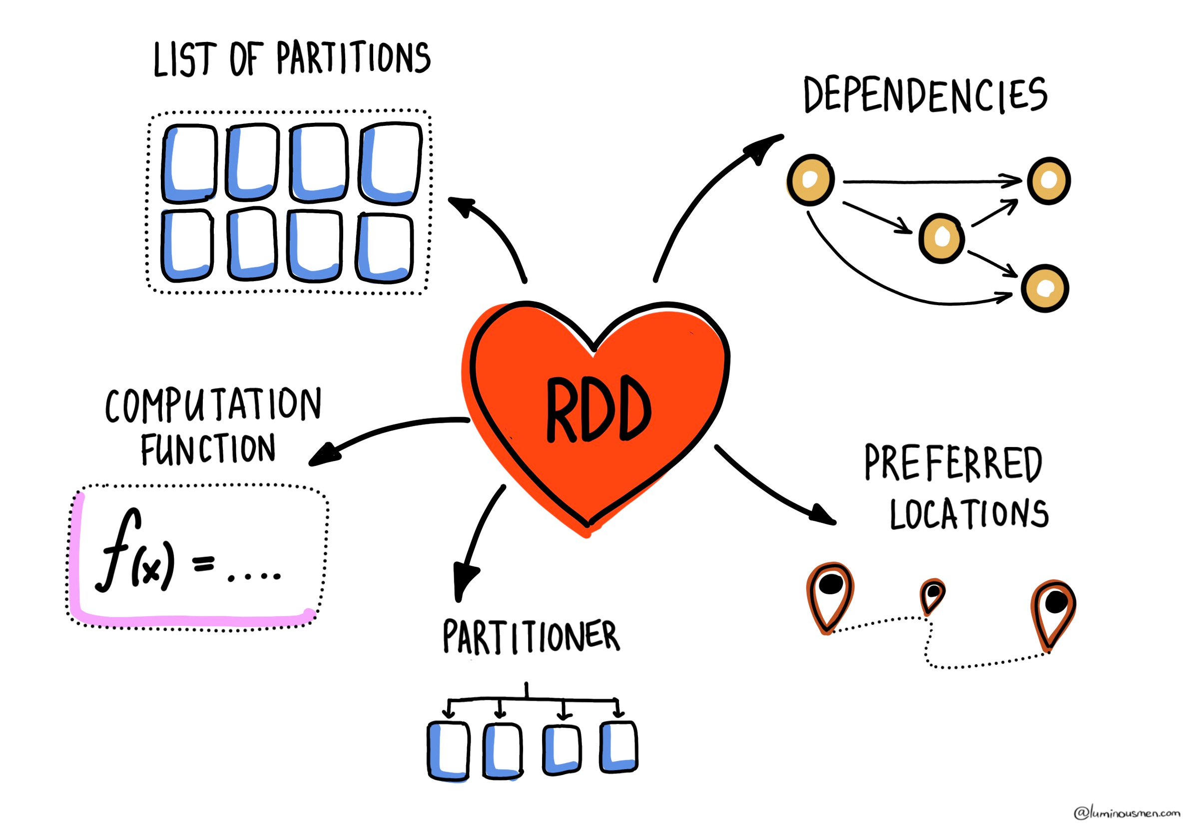
Physically, an RDD lives as an object in the JVM, pointing to data from external sources (HDFS, S3, Cassandra, etc). Every RDD carries its own metadata to enable fault tolerance and distributed execution. Key components include:
Partitions — chunks of data distributed across the cluster nodes. One partition = one unit of parallelism.
Dependencies — lineage information, a list of parent RDDs and transformation history, forming a lineage graph. This lets Spark recompute lost data.
Computation — the computation function applied to parent RDDs.
Preferred Locations — hints where partitions are stored, enabling data-local execution.
Partitioner — defines how data is split into partitions (like default HashPartitioner or RangePartitioner, etc).
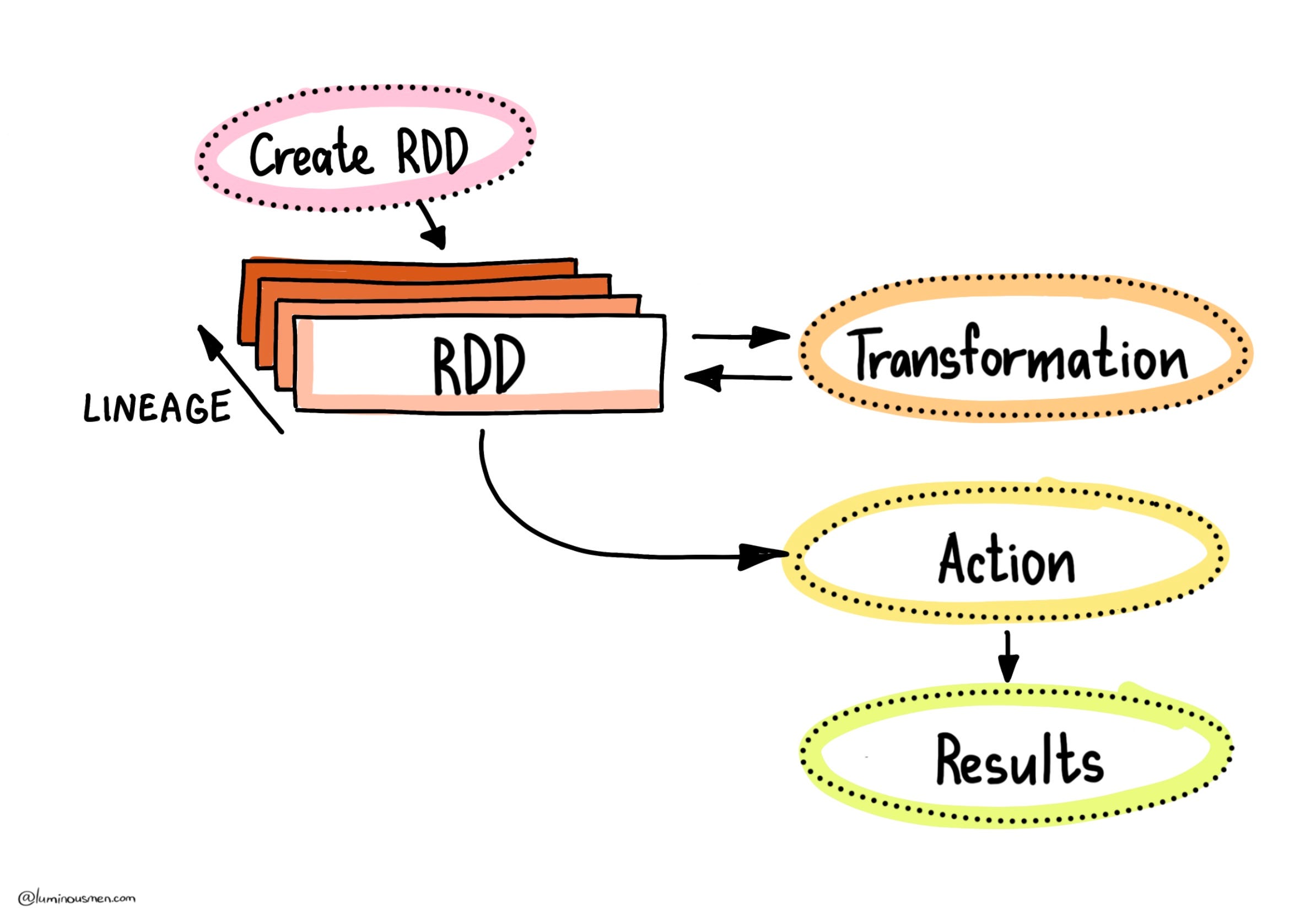
RDDs are immutable — you can never change an RDD in place, you simply derived from an existing RDD using transformation. That new RDD contains a pointer to the parent RDD and Spark keeps track of all the dependencies between these RDDs via lineage graph. In case of data loss, Spark replays the lineage to regenerate it from the original data source making the pipelines fault tolerant.
Here's a quick example:
>>> from pyspark import SparkContext
>>> sc = SparkContext.getOrCreate() # sc is the SparkContext, the entry point to Spark
>>> rdd = sc.parallelize(range(20)) # Create RDD with numbers from 0 to 19
>>> rdd
ParallelCollectionRDD[0] at parallelize at PythonRDD.scala:195
>>> rdd.collect() # Collects all data from nodes and returns it to the driver node
[0, 1, 2, 3, 4, 5, 6, 7, 8, 9, 10, 11, 12, 13, 14, 15, 16, 17, 18, 19]
💡 The Spark Driver orchestrates Spark jobs, manages tasks, and collects results from executors (like with collect()). For a deeper content, check out the next blog post.
RDDs can be cached to optimize repeated computations. This is huge when your pipeline hits the same RDD multiple times. Without caching, Spark must traverse the lineage graph to recompute RDDs from scratch every time they used in a computation.
You can control partitioning manually to balance workloads or rely on Spark's defaults (typically based on cluster configuration). More, smaller partitions often mean better resource utilization (though there's a point of diminishing returns).
Let's inspect the number of partitions and their contents:
>>> rdd.getNumPartitions() # Returns the number of partitions (default behavior depends on cluster settings)
4
>>> rdd.glom().collect() # Collects partitioned data as lists back to the driver node (this is Spark's standard behavior)
[[0, 1, 2, 3, 4], [5, 6, 7, 8, 9], [10, 11, 12, 13, 14], [15, 16, 17, 18, 19]]
All operations on RDDs fall into two categories:
Transformations (lazy)
Actions (eager)
Transformations
Transformations are the backbone of RDD processing in Spark. They're how you take a dataset and do something meaningful with it — filter it, map over it, join it, whatever. But there's a catch: transformations are lazy.
When you call a transformation (e.g. map or filter), Spark doesn't immediately execute it. It just takes notes — "Okay, when someone asks for the result, I'll know what to do". And actual execution only kicks in when you trigger an action like collect or count. This approach — known as lazy evaluation — lets Spark analyze your entire workflow, optimize execution plans, and minimize data movement before doing any heavy lifting.
⚠️ Side effects in transformations? Bad idea. Since transformations are lazy, they might get evaluated multiple times or in weird orders. If you're relying on side effects (like writing to a file in map()), you're setting yourself up for trouble. Just don't.
But not all transformations are created equal. Spark draws a very important line in the sand.
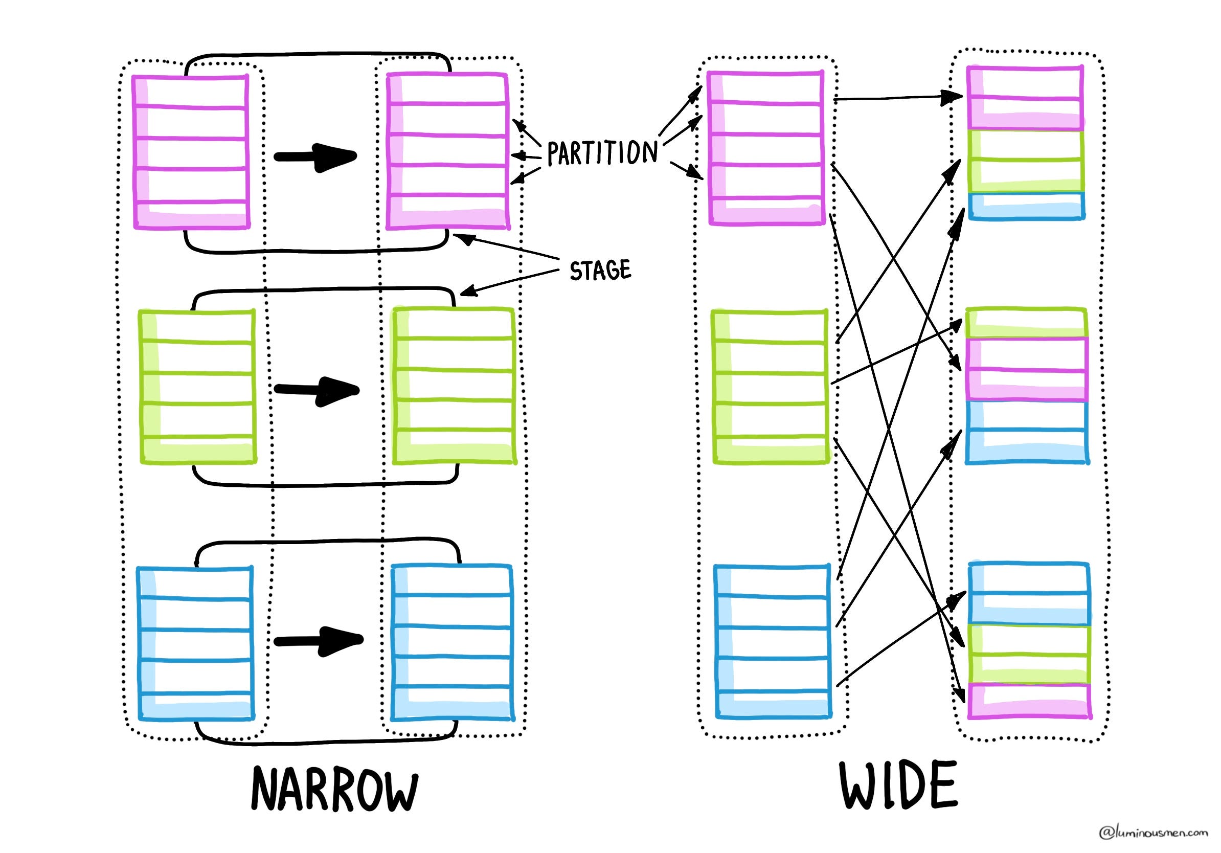
Narrow vs Wide Transformations
Narrow transformations (e.g. map, filter, flatMap) don't require moving data between partitions. Each partition works with its own local data, independently, making these operations fast and highly parallelizable (aka embarrassingly parallel).
Wide transformations (e.g. groupByKey, reduceByKey, join) require shuffling — a fancy way of saying Spark needs to move data between executors to regroup things to meet the transformation's requirements. These are slow, expensive, and should be treated with suspicion unless absolutely necessary.
💡Note on shuffling (aka data shuffle)
A shuffle happens when Spark has to move data between partitions across the cluster — usually to regroup, sort, or aggregate it. This is required when the output of a transformation depends on records from multiple partitions — for example, summing all values or grouping records by some key.
During a shuffle, Spark performs a full-on data exchange: it reads from all partitions, redistributes data according to some partitioning logic, and writes new partitions — often on different executors. That's expensive, as it involves network I/O, data serialization, and disk writes.
Minimizing unnecessary shuffling is key to optimizing Spark jobs.
Narrow transformations operate entirely within a single partition, avoiding the overhead of data shuffling.
For example:
>>> filteredRDD = rdd.filter(lambda x: x > 10) # Filter elements greater than 10
>>> print(filteredRDD.toDebugString()) # Print out the lineage/DAG
(4) PythonRDD[1] at RDD at PythonRDD.scala:53 []
|  ParallelCollectionRDD[0] at parallelize at PythonRDD.scala:195 []
>>> filteredRDD.collect() # Only local partition filtering, no shuffle
[11, 12, 13, 14, 15, 16, 17, 18, 19]
There is no shuffle here — Spark doesn't move any data — each partition filters its own elements. That's what makes narrow transformations cheap and parallelizable. In fact, Spark often fuses a chain of narrow transformations into a single block (a stage), optimizing them behind the scenes.
Wide transformations by contrast involve dependencies across multiple partitions, requiring Spark to shuffle data around. For example:
>>> groupedRDD = filteredRDD.groupBy(lambda x: x % 2) # Group data based on mod
>>> print(groupedRDD.toDebugString()) # Triggers shuffle, costly but necessary for grouping
(4) PythonRDD[6] at RDD at PythonRDD.scala:53 []
|  MapPartitionsRDD[5] at mapPartitions at PythonRDD.scala:133 []
|  ShuffledRDD[4] at partitionBy at NativeMethodAccessorImpl.java:0 []
+-(4) PairwiseRDD[3] at groupBy at <ipython-input-5-a92aa13dcb83>:1 []
|  PythonRDD[2] at groupBy at <ipython-input-5-a92aa13dcb83>:1 []
|  ParallelCollectionRDD[0] at parallelize at PythonRDD.scala:195 []
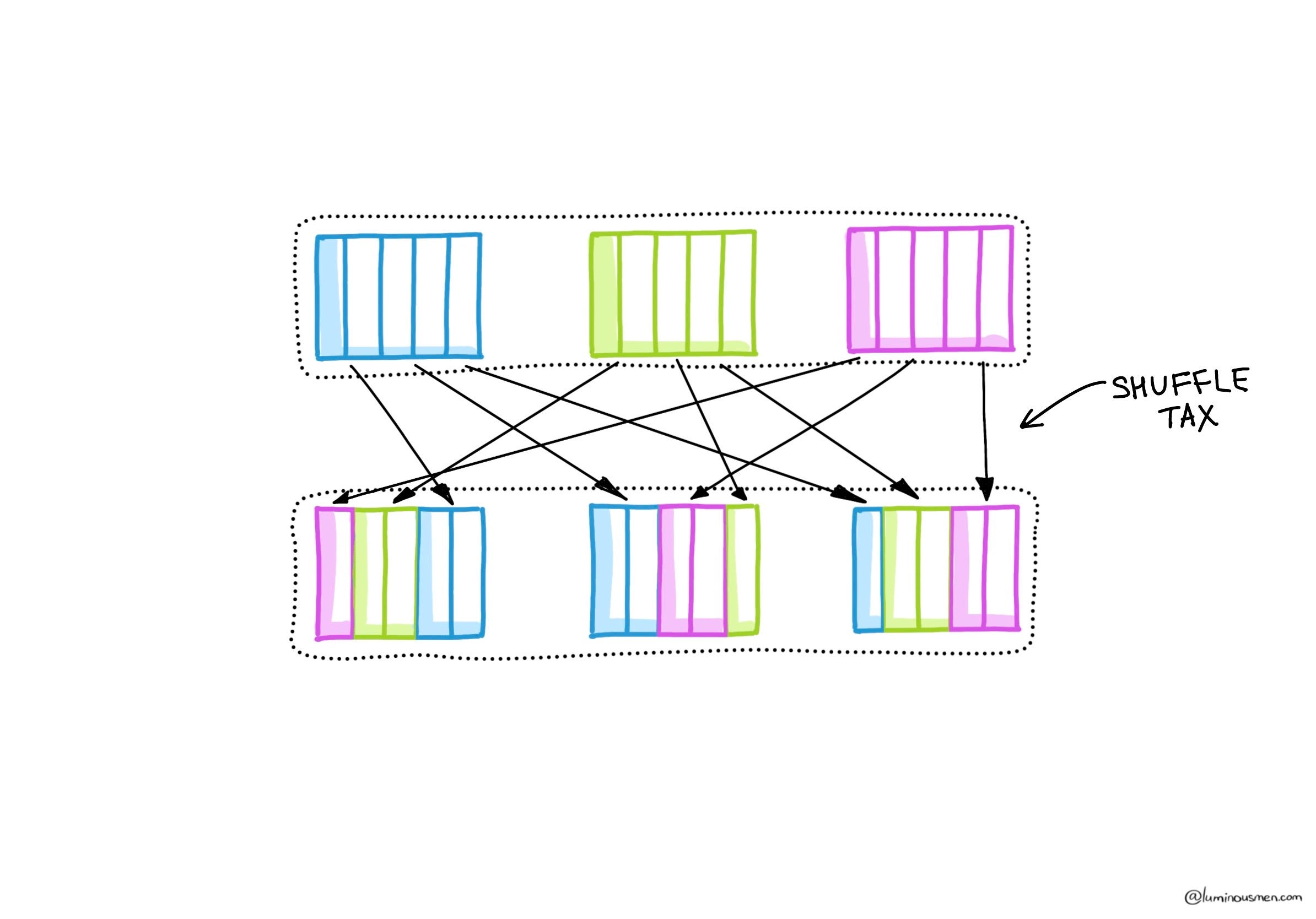
Here, Spark had to shuffle data based on the grouping key (in this case, odd/even values). Notice the ShuffledRDD? That's your performance tax right there.
💡 So when do you have to use wide transformations? If you're grouping, aggregating, or joining across partition boundaries or your logic inherently needs a global view of the dataset. That's fine — just be intentional about it. Know when you're paying the shuffle tax, and make sure it is worth it.
Blog | luminousmen is a reader-supported publication. To receive new posts and support my work, consider becoming a free or paid subscriber.
Actions
Unlike transformations, actions are eager. They will compute things. If transformations are the instructions, actions are the "Go!" button. They're what finally force Spark to roll up its sleeves, stop being lazy, and actually execute the computation.
Calling an action triggers execution of the entire DAG you've been building with transformations. Spark spins up tasks, shuffles data if needed, and materializes the result — whether that means dumping it to disk, loading it into a database, or just printing a sample to console.
Common actions include:
collect: Pulls all the data to the driver. Great for debugging, terrible for large datasets. Don't use it unless you know your data fits in memory.
reduce: Aggregates all elements using a user-defined function.
count: Counts all the elements in the RDD.
For example:
>>> filteredRDD.reduce(lambda a, b: a + b)
135
This line kicks off a full DAG execution. All previous transformations get evaluated, partitioned tasks are distributed across the cluster, and the final result comes to the Spark driver.
Beyond RDDs: DataFrames and Datasets
While RDDs form the foundation of Spark, modern APIs like DataFrames and Datasets are preferred for handling structured data due to their optimizations and simplicity. Here's a quick comparison:
RDDs: Provide low-level control over distributed data but lack query optimizations. Best for unstructured data and fine-grained transformations.
DataFrames: Represent data in a table-like format with named columns (like a SQL table). They leverage Spark's Catalyst Optimizer for efficient query planning and execution.
Datasets: Offer the benefits of DataFrames with type safety, making them ideal for statically typed languages like Scala or Java.
Since Spark 3.x, DataFrames aren't just preferred — they're practically mandatory for performance-sensitive or production Spark workloads. While RDDs give more control, if you're using RDDs for anything besides niche low-level operations, you're fighting the engine.
Directed Acyclic Graph
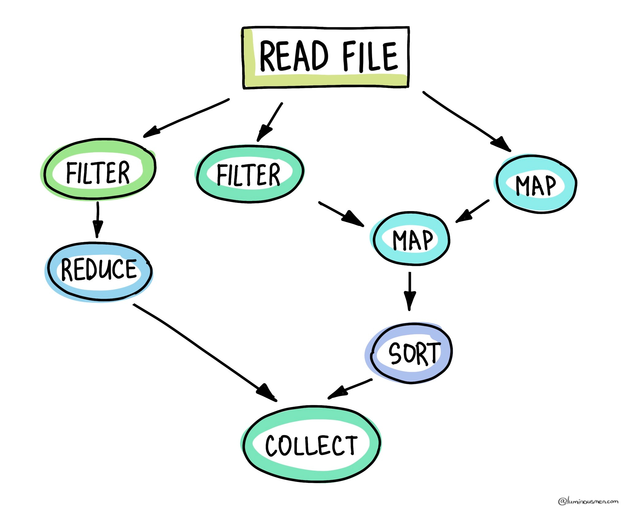
One of the biggest innovations that sets Apache Spark ahead of Hadoop MapReduce — aside from being 100x faster and 10x less painful — is the way it models your computation. Instead of rigid, hardcoded pipelines of Map → Shuffle → Reduce, Spark builds a Directed Acyclic Graph (DAG) as it ingests your transformations: a blueprint of operations and dependencies that spells out exactly how your job will execute.
What Is a DAG, Anyway?
At its core, a DAG in Spark is just a graph with two key properties:
Directed: every edge points one way — there's a clear "before" and "after"
Acyclic: there are no cycles — once you move forward, you cannot loop back
Why does this matter? Because it guarantees that your data processing pipeline has a clear beginning and end. There's no chance of infinite loops, no ambiguous backtracking — just a straight‐line (albeit branching and merging) flow from raw data to final results.
Nodes in this graph are your RDD transformations and actions: map, filter, flatMap, reduceByKey, and so on.
Edges represent the dependencies between those operations: "I can't run this reduceByKey until the map and filter that precede it have finished."
That's it. Simple and elegant.
Logical vs Physical Plans
Before we get into the DAG construction, let's clarify two concepts:
Logical DAG: The abstract plan Spark builds when you define transformations but haven't yet called an action. It's a high‐level blueprint that says "do map, then filter, then reduceByKey", but it hasn't decided how or where to execute anything.
Physical execution plan: The concrete realization of that DAG once you call an action. Here, Spark chooses the actual algorithms, the number of partitions, which nodes to run on, and so forth.
Spark keeps these two worlds separate to maintain laziness — it only pays the execution cost when you truly need a result.
DAG Construction
When you define a chain of transformations nothing executes yet. Spark's driver program records each call, building up that logical DAG in memory. These nodes and edges stack up until you finally call an action - the green light for Spark to convert the logical DAG into a physical execution plan and start processing.
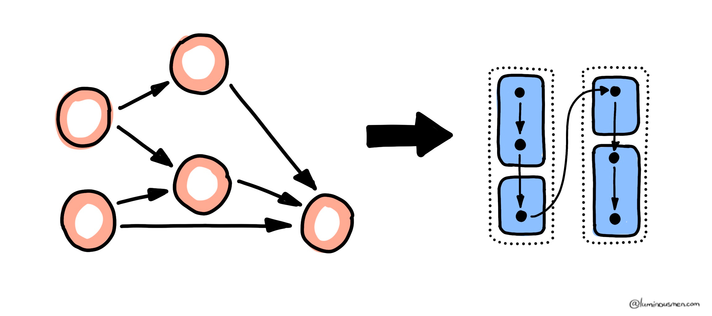
But before Spark can start processing, the logical DAG must be split into stages. A stage is a sequence of operations that can be executed without a shuffle. Narrow transformations like map, filter, and flatMap — process data locally on each partition, so Spark fuses them into the same stage. The moment a wide transformation appears - such as reduceByKey, groupByKey, or join — a shuffle is required, and Spark cuts the DAG, starting a new stage.
Check out this classic word-count example:
sc = SparkContext.getOrCreate()
text = sc.textFile("hdfs://...") # Read text file
words = text.flatMap(lambda line: line.split(r"\s+")) # Split lines into words
pairs = words.map(lambda word: (word, 1)) # Map each word to (word, 1)
counts = pairs.reduceByKey(lambda a, b: a + b) # Reduce by key (word) to get counts
That's two stages, each of which Spark can schedule independently, as soon as its dependencies are met.
Why Spark Builds a DAG
Imagine you're using classic Hadoop MapReduce. You write one Map job, it writes to disk, then a Reduce job reads from disk, does its work, and writes to disk again. On each step, the framework forces you to materialize data to HDFS, incurring heavy I/O and disk seeks. To make matters worse, you have zero understanding into the global structure of your computation — you only see one stage at a time.
Spark's approach — don't run a thing until you have to. Record your intentions, compile them into a DAG, then optimize across the whole graph before you fire off any tasks. That gives Spark two massive advantages:
Global optimization. The DAG allows Spark to treat your code as a full graph, not just a sequence of steps. It sees the entire dependency chain and can make both global and local optimizations — like reordering operations, collapsing stages, or adjusting partitioning dynamically (especially with AQE enabled).
Fault tolerance via lineage. Because Spark knows the entire history of your operations, if a partition goes missing, it only recomputes the lost data by re‐applying the minimal needed transformations — not full job restarts.
The DAG-based execution model is a big reason why Spark can handle complex workloads across massive datasets while minimizing the overhead typically associated with distributed processing. Without the DAG, Spark would lose much of its flexibility, speed, and fault tolerance.
Conclusion
By now you've seen how Spark's core abstractions — RDDs, transformations and actions, and the DAG execution model — work together to deliver both performance and resilience. You know now that lazy evaluation lets Spark optimize across your entire workflow, that narrow transformations avoid costly shuffles, and that lineage‐based fault tolerance keeps your jobs reliable.